The Rejection Rate of ML-DSA Signing: Correcting FIPS-204
Cryptography
Author
Kris Kwiatkowski
Published
October 2, 2026
Introduction
FIPS-204 [1] Table 1 provides the expected number of iterations of the ML-DSA signing loop. Appendix C of the same document uses those figures to derive a loop bound for implementations that choose to impose one. Measurement says the true iteration counts are closer to 4.36, 5.14 and 3.91. The discrepancy is small, but it is not noise, and it is not a rounding artefact. It is a scoping error that happened in translation from the CRYSTALS-Dilithium specification [2] into the standard, and it propagates into every performance figure derived from Table 1 - expected latency, energy budgets, percentile planning, and the loop bound itself.
This post works through where the error comes from and computes the correct values from first principles. The short version:
The figures in Table 1 of [1] account for one of the two rejection points in the signing loop.
The missing one is a consequence of public-key compression, not of security. That is plausibly why a number computed for the security analysis was reused as a performance number.
Correcting it changes the expected iteration counts by 1-2%, and moves the Appendix C loop bound from 814 to 820.
Nothing here affects the security of ML-DSA. The rejection sampling still does what the security proof needs it to do; only the published cost of it is wrong.
This post is the companion analysis referenced from the IETF draft Adapting Constrained Devices for Post-Quantum Cryptography[3], and supplies the numbers used in Benchmarking ML-DSA Signature Generation[4].
NoteCredit
The discrepancy was first reported on pqc-forum by Hanno Becker, with analysis from Markku-Juhani Saarinen, and had been observed earlier in measurements by Mike Hamburg and colleagues in March 2024. This post is an independent derivation that arrives at the same values.
Where the Loop Actually Rejects
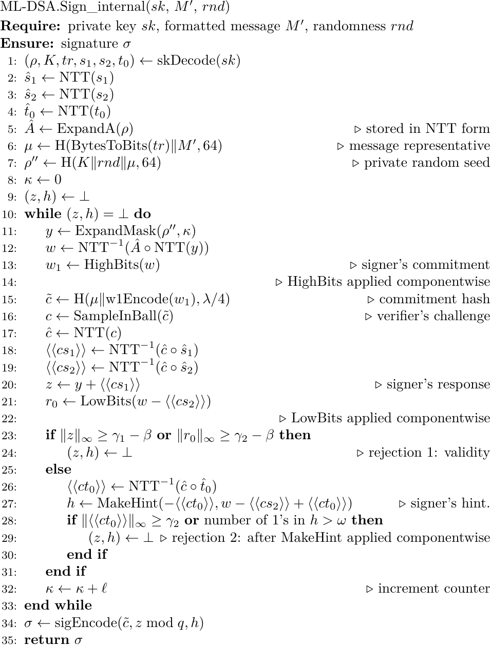
ML-DSA is built on Fiat-Shamir with Aborts. A signing attempt produces a candidate signature, checks it against several bounds, and throws the whole attempt away if any bound is violated. Algorithm 7 of [1] has this shape, with irrelevant lines elided:
ML-DSA signing process
Note the structure: lines 25-28 sit inside the else branch. They are reached only by attempts that already survived line 23. This turns out to matter a great deal later.
There are four rejection conditions in total, and they fall into two quite different categories:
Line
Condition
Character
23
\(\lVert z \rVert_\infty \ge \gamma_1 - \beta\)
security-mandatory
23
\(\lVert r_0 \rVert_\infty \ge \gamma_2 - \beta\)
security-mandatofry
28
\(\#\{i : h_i = 1\} > \omega\)
encoding (compression)
28
\(\lVert c \cdot t_0 \rVert_\infty \ge \gamma_2\)
hint correctness (compression)
Table 1: The four rejection conditions of ML-DSA.Sign_internal.
The two on line 23 are required for the scheme to be secure. Without them the distribution of \(z\) would depend on the private key \(s_1\), and an attacker watching signatures could recover it. The rejection is exactly what makes the output distribution independent of the secret - it is the “Aborts” in Fiat-Shamir with Aborts.
The two on line 28 have nothing to do with security. ML-DSA publishes only the high part of \(t\), dropping \(d = 13\) low bits into \(t_0\), and the signer must transmit hints so the verifier can reconstruct what was dropped. If an attempt needs more hints than the signature format reserves room for, the signature is perfectly secure but cannot be encoded, so it gets discarded. The fourth condition similarly protects the correctness of the hint mechanism.
The Dilithium [2] specification was careful about this. It describes the quantity as “the probability that Step 21 passes”, and labels the corresponding row of its Table 2 “Repetitions (from Eq. (5))”. It also mentions the second rejection point, but bounds it only loosely - “between 1 and 2%” - and gives no formula for it. FIPS-204 reproduced the numbers without the qualifier, stating that Table 1 contains the expected repetitions in the rejection sampling loop of ML-DSA.Sign_internal.
Fixing probability computation
Let’s assume \(p\) is a probability that a single attempt is accepted. Because the checks happen in two groups, with the second evaluated only if the first passed:
where \(P_{norm}\) is the probability of surviving both line-23 checks, \(P_{ct0}\) the probability that \(\lVert c \cdot t_0 \rVert_\infty\) reaches \(\gamma_2\), and \(P_{hint}\) the probability of producing more than \(\omega\) hints. The three terms turn out to need three completely different techniques - exact counting, a closed-form distribution, and simulation - which is most of what makes this interesting.
The Security Checks
Line 23 rejects unless every coefficient of \(z\) and every coefficient of \(r0\) is inside its bound. Both are handled by the same counting argument.
The z check
The condition is \(\lVert z \rVert_\infty \lt \gamma_1 - \beta\) , where \(z = y + c \cdot s1\). Take one coefficient \(z_i = y_i + (c \cdot s_1)_i\). The only randomness is \(y_i\), which \(ExpandMask\) (Algorithm 34, [1]) draws uniformly from \(2 \cdot γ1\) possible values. The permitted range in which \(z_i\) may land in, is an open interval \((-(\gamma_1 - \beta), \gamma_1 - \beta)\), hence there are \(2(\gamma_1 - \beta) - 1 \quad\) admissible values.
This count does not depend on the value of \((c \cdot s_1)_i\). The per-coefficient probability is therefore the same whatever the secret key happens to be:
\[
P(\text{coefficient of } z \text{ passes}) = \frac{2(\gamma_1 - \beta) - 1}{2\gamma_1}
\]
This factor is exact. It is a counting argument over a distribution that is uniform by construction, with no approximation and no assumption.
The \(r_0\) check
The condition is \(\lVert r_0 \rVert_\infty \lt \gamma_2 - \beta\), with \(r_0 = LowBits(w - c \cdot s_2)\) taking one of \(2 \cdot \gamma_2\) possible values. The identical count gives
This factor is not exact. It assumes the low bits of \(w - c \cdot s_2\) are uniformly distributed over their residues. They are not sampled - they are a deterministic function of \(A\), \(y\), \(c\) and \(s_2\) - so this is a modeling assumption (a heuristic), not a derived fact. It is resting on the expectation that modular reduction of a pseudorandom quantity scrambles the low-order bits.
Putting them together
An attempt passes line 23 only if every coefficient passes. One violation anywhere kills the attempt. There are \(256 \cdot l\) coefficients in \(z\) and \(256 \cdot k\) in \(r_0\), treated as independent, so:
from dataclasses import dataclassimport pandas as pdimport math@dataclassclass MLDSAParams: name: str n: int# ring degree, always 256 q: int# modulus tau: int# number of +-1's in the challenge poly c gamma1: int# y coefficient range gamma2: int# low-bits rounding range k: int# rows of A (dimension of w, s2, t) l: int# columns of A (dimension of s1, z) eta: int# secret key coefficient range d: int# dropped bits of t omega: int# maximum number of hints@propertydef beta(self) ->int:returnself.tau *self.eta# FIPS-204 Table 1PARAMS = [ MLDSAParams("ML-DSA-44", n=256, q=8380417, tau=39, gamma1=2**17, gamma2=(8380417-1) //88, k=4, l=4, eta=2, d=13, omega=80), MLDSAParams("ML-DSA-65", n=256, q=8380417, tau=49, gamma1=2**19, gamma2=(8380417-1) //32, k=6, l=5, eta=4, d=13, omega=55), MLDSAParams("ML-DSA-87", n=256, q=8380417, tau=60, gamma1=2**19, gamma2=(8380417-1) //32, k=8, l=7, eta=2, d=13, omega=75),]def p_norm_exact(p: MLDSAParams) ->float:""" This computes probability that both z-check and r0-check passes. Each coefficient of z = y + c*s1 is in the good range for exactly 2(gamma1-beta)-1 of the 2*gamma1 possible y values, independent of the value of the c*s1 coefficient. The r0 term is treated analogously: we assume its low bits are uniformly distributed over their 2gamma2 possible residues, and compute the probability under that assumption. The infinity-norm check requires that every coefficient of z be within gamma1 - beta in absolute value, and every coefficient of r0 be within gamma2 - beta in absolute value. """ g1, g2, b = p.gamma1, p.gamma2, p.beta# Exact norm-check product:# p_norm = [(2(gamma1-beta)-1)/(2 gamma1)]^(256 l)# * [(2(gamma2-beta)-1)/(2 gamma2)]^(256 k) base_z = (2*(g1-b)-1) / (2*g1) # z base_r = (2*(g2-b)-1) / (2*g2) # r0 p_norm = base_z**(p.n*p.l) * base_r**(p.n*p.k)return p_normdef p_norm_eq5(p: MLDSAParams) ->float:"""Equation (5) of the Dilithium spec: first-order approximation."""return math.exp(-256* p.beta * (p.l / p.gamma1 + p.k / p.gamma2))pd.DataFrame([ {"ML-DSA Variant": p.name,r"\(P_{\mathrm{norm}}\)": f"{p_norm_exact(p):.5f}","Equation (5)": f"{p_norm_eq5(p):.5f}","Overstatement": f"{100*(p_norm_eq5(p)/p_norm_exact(p) -1):.1f}%", }for p in PARAMS]).set_index("ML-DSA Variant")
\(P_{\mathrm{norm}}\)
Equation (5)
Overstatement
ML-DSA Variant
ML-DSA-44
0.23272
0.23502
1.0%
ML-DSA-65
0.19539
0.19631
0.5%
ML-DSA-87
0.25809
0.25961
0.6%
Table 2: Probability of passing the line-23 validity checks, per attempt. The exact product is compared against Equation (5) of the Dilithium (v3.1) specification, which approximates it.
Equation (5) of the Dilithium specification is an approximation of this product. Two things are worth separating. It is an approximation, good to about 1%, which the exact product above fixes. And it covers only the line-23 checks, whereas FIPS-204 presents it as the whole loop - which is the larger error, and needs the two remaining terms.
NoteNOTE: Compounding of per-coefficient probabilities
The compounding is worth pausing on, because it is genuinely unintuitive. Each coefficient is rejected with probability well under 0.1% - between roughly one in 1,200 and one in 4,300. But there are between two and four thousand coefficients, and all must pass at once. Since \((1-x)^N \approx e^{-Nx}\) and \(Nx \approx 1.4\), survival collapses to about a quarter. The same compounding explains Equation (5)’s error: a per-coefficient discrepancy of only \(1/(2\gamma)\) - a few parts per million - accumulates over thousands of coefficients into roughly 0.5-1% in \(P_{norm}\).
Two separate problems have now been isolated. Equation (5) is an approximation of \(P_{norm}\), good to about a percent - that is a precision issue, and the exact product fixes it. But Equation (5) is also only\(P_{norm}\), whereas FIPS-204 presents it as the whole loop - that is a scoping issue, and fixing it needs the two remaining terms.
The Hint-Correctness Check
This is the smallest of the three terms, and it has the cleanest answer. It comes before \(P_{hint}\) because both depend on the distribution of a coefficient of \(c \cdot t_0\), which is derived here.
What the check does
ML-DSA compresses its public key. The full value \(t = A \cdot s_1 + s_2\) is split by \(Power2Round\) (Algorithm 35 of FIPS-204 [1]) into a high part \(t_1\), which is published, and a low part \(t_0\), which is not. The verifier therefore cannot compute the high bits of \(A \cdot z - c \cdot t\) directly, and the signer sends hints recording where the missing \(c \cdot t_0\) term causes a carry across a high-bit boundary.
The verifier does not know \(t_0\), so the value it computes is off by \(c \cdot t_0\). One hint bit per coefficient can correct this only if \(c \cdot t_0\) is small enough that it never carries a coefficient more than one high-bits boundary away. The governing lemma makes this precise: each coefficient of \(c \cdot t_0\) must be at most \(\alpha/2 = \gamma_2\) in absolute value. So before trusting the hint, the signer checks \(\lVert c \cdot t_0 \rVert_\infty < \gamma_2\), and if the check fails it discards the attempt, because the signature might not verify.
The distribution of a coefficient of \(c \cdot t_0\)
\(Power2Round\) defines \(t_0 = t \bmod^{\pm} 2^d\), where \(\bmod^{\pm}\) is the centred representative. So the coefficients of \(t_0\) lie in
That is \(2^d = 8192\) consecutive integers, centred on zero. The centring is not incidental - it makes the distribution essentially zero-mean, which is what lets \(c \cdot t_0\) be treated as a zero-mean sum. Assuming these coefficients are uniform over their 8192 values, the variance of a uniform over \(N\) consecutive integers is \((N^2-1)/12\), so
The challenge polynomial \(c\), produced by \(SampleInBall\) (Algorithm 29 of FIPS-204 [1]), has exactly \(\tau\) non-zero coefficients, each \(+1\) or \(-1\), the rest zero. So each coefficient of the product \(c·t_0\) is a signed sum of exactly \(τ\) coefficients of \(t_0\).
Two facts about this sum matter.
Its spread. Each coefficient of \(c \cdot t_0\) adds up \(\tau\) independent coefficients of \(t_0\), so their variances add:
That is 14768, 16554 and 18318 for the three parameter sets - a typical coefficient of \(c \cdot t_0\) is in the tens of thousands. The threshold \(\gamma_2\) is 6.4, 15.8 and 14.3 times larger than that, so the check rarely fails. But \(\sigma\) alone does not say how rarely.
Its range. Each term is at most \(2^{d-1} = 4096\) in absolute value, so
\[|(c \cdot t_0)_i| \le \tau \cdot 2^{d-1}\]
which is 159744, 200704 and 245760. For ML-DSA-65 and ML-DSA-87 this maximum is below \(\gamma_2 = 261888\): the check cannot fail, and \(P_{ct_0} = 0\) exactly. For ML-DSA-44 the maximum exceeds \(\gamma_2 = 95232\), so the tail has to be computed.
Irwin-Hall distribution
A sum of uniform variables is, by definition, Irwin-Hall distributed. Not approximately - exactly. And unusually for a continuous distribution, its CDF has a closed form:
Its support is bounded - \(IH_n\) lies in \([0, n]\) and nowhere else - which is precisely what the normal approximation lacks.
The sum above is finite and directly computable.
The signs of \(c\) can be ignored, since the uniform range is symmetric about zero and negating a symmetric variable leaves its distribution unchanged. Rescaling by the interval width \(2^d\) puts the threshold at \(x = \frac{\gamma_2}{2^d} + \frac{\tau}{2}\) in Irwin-Hall units.
threshold x
IH support
P_ct0
ML-DSA Variant
ML-DSA-44
31.12
[0, 39]
7.33e-09
ML-DSA-65
56.47
[0, 49]
0
ML-DSA-87
61.97
[0, 60]
0
Table 3: P_ct0, computed exactly via the Irwin-Hall distribution. For ML-DSA-65 and ML-DSA-87 the threshold falls outside the support of the distribution, so the tail is exactly zero.
One calculation, no special cases. For ML-DSA-65 and ML-DSA-87 the threshold lands beyond the support of the distribution - 56.47 against a maximum of 49, and 61.97 against a maximum of 60 - and the tail beyond the support of a distribution is exactly zero. The condition cannot fire at all for those parameter sets.
The same result without any distribution
Those two zeros can be had more directly, and on weaker assumptions. Since \(|(c \cdot t_0)_i| \le \tau \cdot 2^{d-1}\) always:
Variant
\(\tau \cdot 2^{d-1}\)
\(\gamma_2\)
Can the check fire?
ML-DSA-44
159,744
95,232
yes
ML-DSA-65
200,704
261,888
no
ML-DSA-87
245,760
261,888
no
Table 4: Support bound against threshold.
For ML-DSA-65 and ML-DSA-87 the largest value \(c \cdot t_0\) can possibly attain is below the threshold, so the condition is unsatisfiable. This is the same fact as “x exceeds the Irwin-Hall support”, stated in unscaled units - not a different method. Its value is that it holds for any \(t_0\) in the valid range, and so does not depend on the uniformity assumption at all. The ML-DSA-44 figure, by contrast, does.
In theory, this check could be skipped for MLDSA-65 and -87, in practice not sure that would be FIPS-approved.
The Hint-Weight Rejection
This is the term FIPS-204 omits entirely, and the larger of the two missing corrections.
What needs to be computed
Line 26 of the algorithm, computes a vector of hints, one bit per coefficient, so \(h\) holds \(256 \cdot k\) bits. Line 28 rejects when the number of 1 bits exceeds \(\omega\) - the number of hint positions the signature format reserves space for. Writing \(N\) for that count:
\[
P_{hint} = P(N > \omega)
\]
Notice what kind of object this is. \(P_norm\) and \(P_{ct_0}\) each concerned a single quantity crossing a threshold. Here the question is about a count of events across thousands of coefficients. That is a structurally harder problem, and it is why this term resisted a closed-form treatment.
Condition to fire single hint
\(\mathrm{MakeHint}(z, r)\) returns 1 when \(\mathrm{HighBits}(r)\) differs from \(\mathrm{HighBits}(r + z)\). Line 26 invokes it as
\[
h = \mathrm{MakeHint}(-c \cdot t_0,\ w - c \cdot s_2 + c \cdot t_0)
\]
so \(r = w - c \cdot s_2 + c \cdot t_0\) and \(r + z = w - c \cdot s_2\). A hint at position \(i\) therefore fires exactly when adding \((c \cdot t_0)_i\) changes the high bits of \((w - c \cdot s_2)_i\) - that is, when its low part is pushed out of \((-\gamma_2,\ \gamma_2]\).
That low part is \(r_0\), the very quantity checked on line 23. And here the structure of the algorithm matters. Lines 25-28 live inside the else branch, reached only when line 23 already passed. So by the time hints are computed, \(r_0\) is not free to take any value in \((-\gamma_2,\ \gamma_2]\); it is already confined to \(|r_0| < \gamma_2 - \beta\), a narrower range.
Counting admissible values of \(r_0\) exactly, with \(a = |(c \cdot t_0)_i|\) and \(r_0\) uniform over the \(2(\gamma_2 - \beta) - 1\) values line 23 permits: for \(a > 0\) the hint fires when \(r_0\) exceeds \(\gamma_2 - a\), which happens for \(\max(0,\ a - \beta - 1)\) of them. The opposite side is unreachable. So
\[
P(\text{hint at } i \mid |(c \cdot t_0)_i| = a) = \frac{\max(0,\ a - \beta - 1)}{2(\gamma_2 - \beta) - 1}
\]
Two consequences. No hint is possible at all unless \(|(c \cdot t_0)_i|\) exceeds \(\beta\). And the expression one would write without noticing the conditioning - \(a / (2\gamma_2)\) - overstates the hint rate by roughly 10 to 30 percent depending on parameter set.
Monte Carlo
Each trial simulates one signing attempt that has already passed line 23:
sample \(c\): \(\tau\) positions among 256, each \(\pm 1\), rest zero
sample \(t_0\): \(k\) polynomials of 256 coefficients, uniform on \((-2^{d-1},\ 2^{d-1}]\)
compute \(c \cdot t_0\) in \(\mathbb{Z}[X]/(X^{256}+1)\)
for each of the \(256 \cdot k\) coefficients, compute its hint probability and draw the Bernoulli outcome
\(N\) = number of hints; record whether \(N > \omega\)
\(P_{hint}\) is the fraction of trials in which \(N\) exceeded \(\omega\). The product in step 3 is computed by negacyclic FFT: weight both operands by \(\exp(i \pi j / 256)\), do an ordinary cyclic convolution, unweight. Values stay below \(\tau \cdot 2^{d-1} = 245{,}760\), far under \(q/2\), so no modular reduction is needed and double precision is amply accurate. A direct sparse convolution is correct but about two orders of magnitude slower, which matters when you need hundreds of thousands of trials.
mean hint count
omega
P_hint
ML-DSA Variant
ML-DSA-44
63.0
80
0.01464 ± 0.00016
ML-DSA-65
38.2
55
0.00374 ± 0.00008
ML-DSA-87
56.7
75
0.00775 ± 0.00011
Table 5: P_hint, estimated by Monte Carlo. 600,000 trials per parameter set, reproduced under independent seeds; the stated uncertainty is the binomial standard error.
The mean hint counts sit comfortably below \(\omega\) in every case - the parameter sets were chosen that way - and it is only the upper tail of the count that spills over. Two sanity checks came out right: the simulated means match the analytic prediction, and the simulation recorded zero occurrences of the \(\lVert c \cdot t_0 \rVert_{\infty} \ge \gamma_2\) condition across 1.8 million attempts, consistent with the \(P_{ct_0}\) figures above.
Results
Putting the three terms together:
P_norm
P_ct0
P_hint
p
1/p
measured
FIPS-204
ML-DSA Variant
ML-DSA-44
0.23272
7.3e-09
0.01464
0.22932
4.361
4.358
4.25
ML-DSA-65
0.19539
0
0.00374
0.19466
5.137
5.137
5.1
ML-DSA-87
0.25809
0
0.00775
0.25609
3.905
3.905
3.85
Table 6: Per-attempt acceptance probability and expected iteration count, against the figures published in FIPS-204 Table 1 and against independent measurement.
The derived values agree with independent measurement to 0.06%, 0.003% and 0.002%. That agreement is the real evidence that the modelling assumptions - the two uniformity heuristics and the independence assumptions in the Monte Carlo - are adequate at this precision. None of them is provable; all of them are testable, and they pass.
Everything downstream is now just the geometric distribution evaluated at these values of p.
ML-DSA-44
ML-DSA-65
ML-DSA-87
Iterations
1
22.93%
19.47%
25.61%
2
40.60%
35.14%
44.66%
3
54.23%
47.77%
58.83%
4
64.72%
57.94%
69.37%
5
72.81%
66.12%
77.22%
6
79.05%
72.72%
83.05%
7
83.85%
78.03%
87.39%
8
87.55%
82.31%
90.62%
9
90.41%
85.75%
93.02%
10
92.61%
88.52%
94.81%
11
94.30%
90.76%
96.14%
12
95.61%
92.56%
97.13%
Table 7: Probability of completing the signing process within a given number of iterations.
ML-DSA-44
ML-DSA-65
ML-DSA-87
Target
90%
9
11
8
95%
12
14
11
99%
18
22
16
Table 8: Iterations required to reach a given probability of completing the signing process.
Every variant reaches at least 90% within 11 iterations, but the tail runs long. ML-DSA-65 needs 22 iterations to reach 99%.
Verifier
The agreement claimed above is the load-bearing evidence for the modelling assumptions, so it should not have to be taken on trust. The panel below runs mldsa-ref [5] compiled to WebAssembly and measures the acceptance probability in your browser, against the derived value from the table above.
Loading WebAssembly…
The key count is the control worth experimenting with. \(P_{hint}\) depends on the key through \(t_0\), so the per-attempt acceptance probability is not identical for every key, and an average taken over too few keys estimates those keys’ value rather than the population’s. That kind of bias does not shrink as you add signatures - it shrinks as you add keys.
A caveat on what this panel can and cannot show. Ten thousand browser signatures give a standard error of roughly 0.04 on the mean - enough to confirm the derived value, not enough to argue with it. The 200,000 setting brings that to about 0.009, which is genuinely useful, at the cost of several minutes of your CPU.
Conclusion
The error in FIPS-204 Table 1 is small in magnitude and entirely benign for security, but it is instructive about how numbers travel between documents.
The Dilithium specification computed the probability it needed for its security argument, scoped the claim correctly, and said so twice - in the surrounding text and in the label of the table row. It also acknowledged the second rejection point, bounded it loosely at “between 1 and 2%”, and never computed it, because it did not need to. Every statement in that document is true.
FIPS-204 needed a different quantity - the cost of the loop, not the probability of one of its checks - and reused the available number. The qualifier did not survive the move. Nobody was careless, the figure was simply asked to answer a question it was never computed for.
References
[1]
National Institute of Standards and Technology, “Module-Lattice-Based Digital Signature Standard,” U.S. Department of Commerce, Federal Information Processing Standards Publication FIPS 204, Aug. 2024. doi: 10.6028/NIST.FIPS.204.
T. Reddy, D. Wing, B. Salter, and K. Kwiatkowski, “Adapting Constrained Devices for Post-Quantum Cryptography,” Internet Engineering Task Force, Internet-Draft draft-ietf-pquip-pqc-hsm-constrained, 2026. Available: https://datatracker.ietf.org/doc/draft-ietf-pquip-pqc-hsm-constrained/